Why a Better Stabilisation Ratio Can Lose

The strongest headline number can lose

A stabiliser can reduce one movement by a factor of 63 and make another movement 50% larger. The calculation in this paper shows how. Its lesson is useful when choosing a camera positioner: a strong result at one test frequency can hide a weak region elsewhere.

An inspection boat makes the question tangible. Waves rock the hull; machinery adds other vibrations. Both reach the camera support, but they need not occur at the same rate. Measuring only the largest visible movement can miss the frequency that controls the final result.

Even equipment used to steady a platform can disturb it. NASA reports that reaction wheels, which turn spacecraft, can also be major sources of pointing vibration through imbalance and bearing noise. The engineering lesson is to include internal machinery in the disturbance record, as well as the environment. NASA technical account

Define the ratio before comparing it

For a steady sinusoidal test, let D be base angular motion and E be residual optical-axis motion relative to a fixed reference, both at the test frequency. Use the same axis, units and amplitude convention.

Rejection ratio R = D / E. Residual gain G = E / D = 1 / R.

A residual gain of 0.1 means one-tenth of the input motion remains. A gain of 1 means no reduction; above 1 means amplification. Frequency response also includes phase: how far the output lags or leads the input. MIT frequency response notes

Keep peak and root-mean-square (RMS) values distinct. For a pure sine wave, RMS equals peak amplitude divided by √2. Mixing the two creates a false advantage before the comparison even starts.

A rejection ratio belongs to a frequency, an amplitude and a defined motion path.

Read the whole response curve

Feedback repeatedly measures motion and commands a correction. Its useful frequency range depends on the actuator, sensors, mechanical structure and controller settings. A response curve shows what remains as the disturbance becomes faster. A single bandwidth number cannot show the shape of that curve.

In a simple negative-feedback loop, an angular disturbance added directly at the output has sensitivity S = 1 / (1 + L), where L is the combined controller and plant response. Large loop gain can reduce this disturbance. Sensor noise enters through a different response, T = L / (1 + L). Increasing correction strength therefore has consequences for noise too. MIT feedback performance notes

Do not automatically label every measured base-to-camera response S. Base rotation, applied torque and sensor noise enter at different places. Their paths through the mechanics and control system differ. For a positioner comparison, request the measured transfer from base angle to optical-axis angle for the intended configuration.

The transition region deserves attention

Correction may arrive with enough delay and phase shift to reinforce motion in a narrow band. In the stable linear models used here, transient motion dies away after the forcing stops. During periodic forcing, the residual can still exceed the input.

A pure 10 ms delay adds 36° of phase lag at 10 Hz, but only 3.6° at 1 Hz: lag = 360 × frequency × delay. This calculation does not establish a stability margin; the rest of the loop matters. MIT frequency response notes

Ask how the response changes with payload inertia, mounting stiffness and operating mode. A curve measured with one payload is evidence for that setup. It is not automatically evidence for every load the positioner can carry.

Combine response with the motion spectrum

For random motion with zero mean and steady statistics, power spectral density (PSD) describes mean-square motion per unit frequency. With a one-sided angular PSD in degrees squared per hertz, multiply by G(f)² and integrate over the stated positive-frequency band. This gives residual mean-square motion; take its square root for degrees RMS. Do not average rejection ratios. MIT spectral analysis notes

Request residual gain and phase across the active band, including any peak above unity.

One spectrum, two different winners

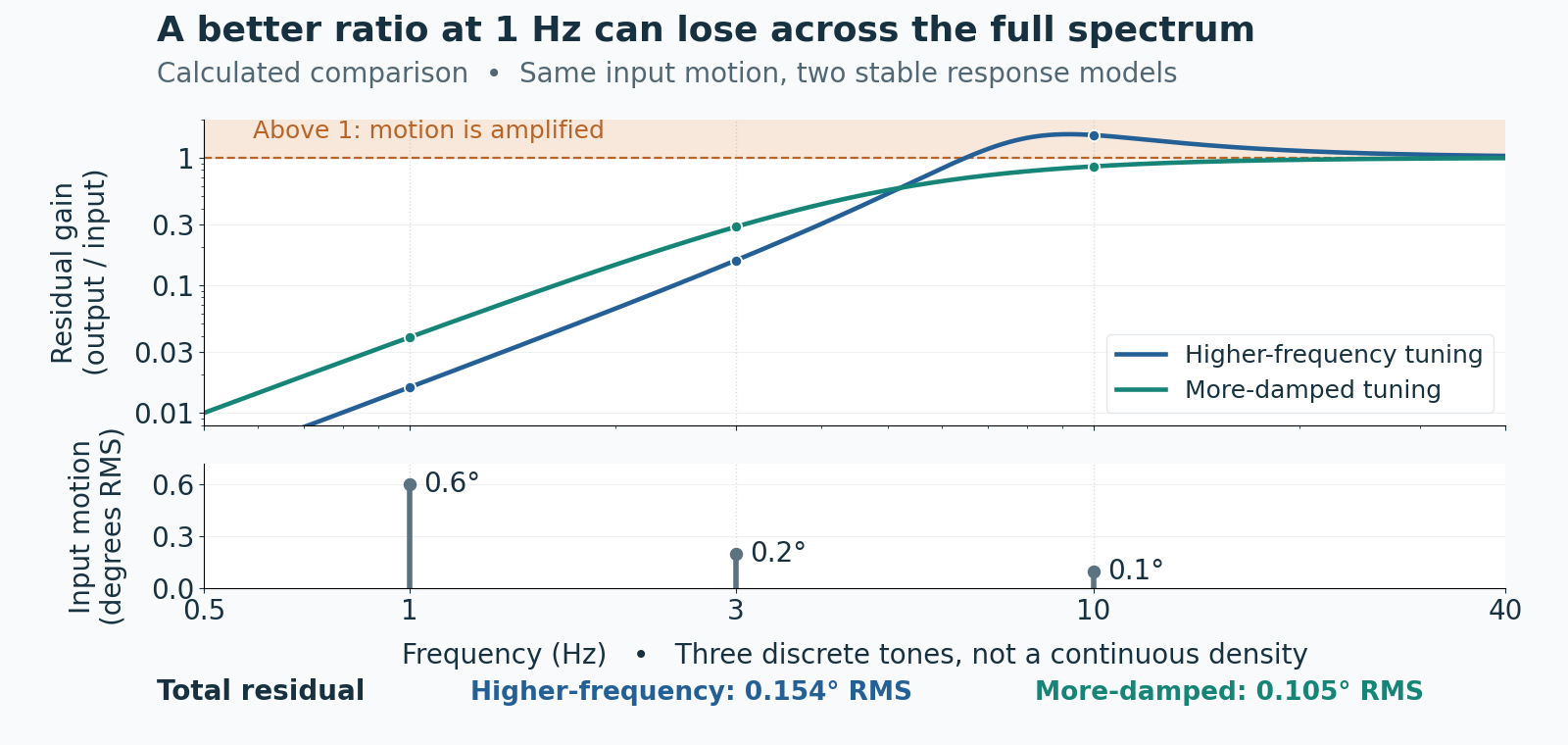
Two calculated residual-gain curves above one three-tone input spectrum. Higher-frequency tuning amplifies the 10 Hz input and leaves more total motion. — Calculated response to the same three inputs: 0.154° RMS versus 0.105° RMS. The 10 Hz component reverses the ranking.

Consider one axis with three sinusoidal base motions: 0.6° RMS at 1 Hz, 0.2° RMS at 3 Hz and 0.1° RMS at 10 Hz. These are assumed inputs for a calculation, not measured product performance. Evaluate two stable linear models, with no added noise or saturation.

The model gain is G = r² / √[(1 − r²)² + (2ζr)²], where r = f / f₀. Higher-frequency tuning uses f₀ = 8 Hz and damping ζ = 0.35; more-damped tuning uses f₀ = 5 Hz and ζ = 0.90. Here f₀ sets the model’s frequency scale; it is not a quoted product bandwidth.

Frequency	Higher-frequency gain	More-damped gain
1 Hz	0.0158	0.0390
3 Hz	0.1565	0.2868
10 Hz	1.5021	0.8536

At 1 Hz, the first model offers about 63:1 rejection against 26:1. Yet its amplification near 10 Hz changes the outcome. Multiply each input RMS value by its gain, square the three results, add them, then take the square root. Over whole cycles, the distinct tones have zero cross terms.

The total residual is 0.154° RMS for higher-frequency tuning and 0.105° RMS for more-damped tuning. The stronger headline ratio leaves about 46% more residual movement.

If the 10 Hz input disappears, the ranking reverses: the totals become 0.0327° and 0.0619° RMS. Neither curve wins independently of the disturbance spectrum.

Weight the response by the motion that actually occurs, rather than averaging rejection ratios.

Turn the curve into useful evidence

An optical camera on a tilting motion table faces a checkerboard target fixed independently to the laboratory floor. — Measure the moving base and the view of an independent reference. Account for lens translation when using a nearby target.

Start with angular motion measured at the intended mounting interface during the operating condition of interest. Record axis, sample rate, filtering, machinery state and duration. Keep quiet periods separate from operating periods that have different vibration sources. When estimating a random-motion spectrum, averaging reduces fluctuations, while shorter data segments reduce frequency resolution. Preserve narrow peaks that may overlap the controller’s weak region. MIT spectral analysis notes

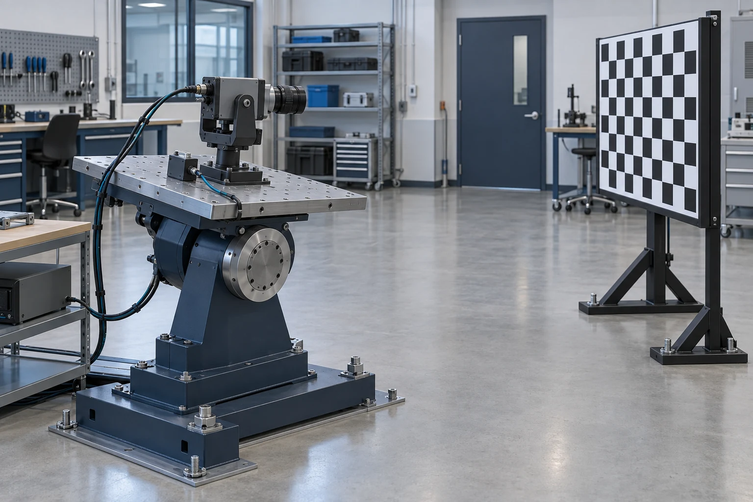
On a motion table, measure base motion and residual optical motion together. A fixed target provides an independent reference. A nearby target can also move in the image because the lens translates. Use a collimated reference, whose optics make a target appear effectively infinitely far away, or correct the measurement geometry. Disable or record image processing that changes the observed motion.

Small-motion results need an amplitude check

A sine movement with peak angle A requires peak rate 2πfA for perfect cancellation. At A = 1° and f = 5 Hz, that is 31.4°/s; the peak acceleration is 987°/s². Doubling frequency doubles required rate and quadruples acceleration. These are kinematic demands, not positioner ratings.

Repeat tests at the intended disturbance amplitude. Rate or torque limits can invalidate a small-motion curve; an integrating controller can also recover slowly after saturation. MIT actuator-limit notes

The Inventra S³ PED12 product page identifies gyro stabilisation and a published stabilisation accuracy of 0.04°. That single angle does not supply the frequency-response evidence used here. Request the response, amplitude, axis and payload conditions for the proposed configuration.

Choose the configuration with acceptable residual motion across the relevant spectrum and sufficient actuator margin. Then check the resulting image with the intended camera settings. The shutter-time lesson and the mechanical line-of-sight budget address the next two questions.

Select against the operating spectrum, then verify the same optical measurement with the intended payload.

Download the full article (PDF)

The Better Stabilisation Ratio Can Give the Worse Result