Positioner Accuracy: What Averaging Cannot Fix

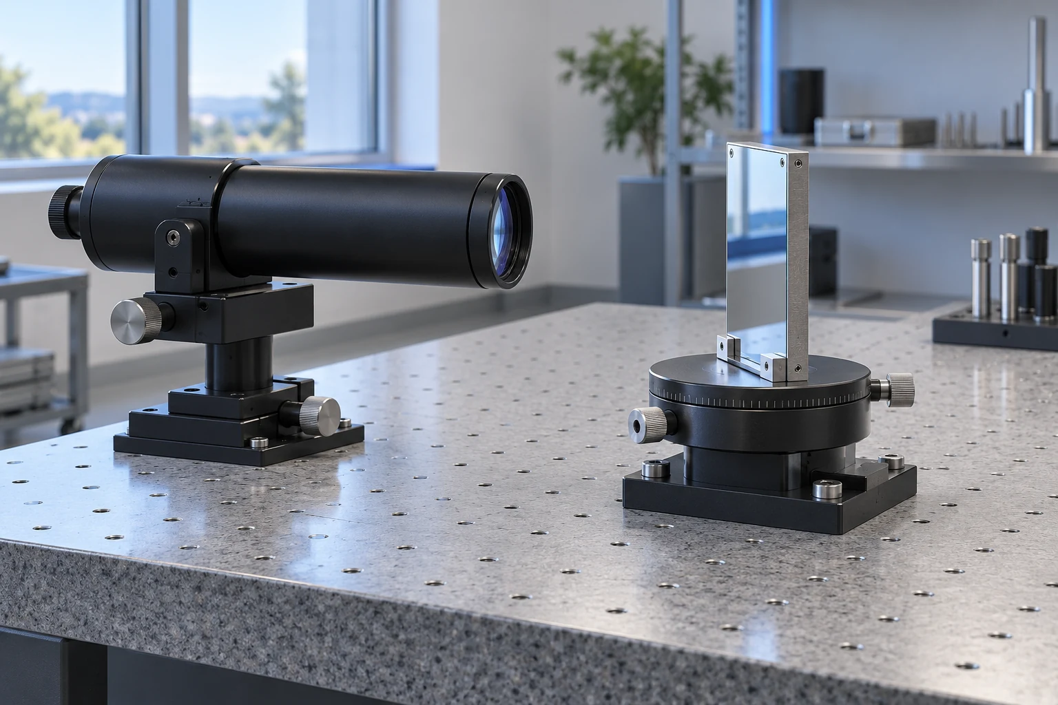
A fine readout can describe the wrong angle

A positioner can report 30.000° every time while the camera consistently points somewhere else. Extra decimal places make the indication look convincing. They do not reveal an offset between that indication and an independent angular reference.

Start by separating five questions. These plain-language descriptions follow the International Vocabulary of Metrology, sections 2.13–2.26 and 4.14.

Term	The question it answers
Resolution	What is the smallest change in the measured quantity that the indication can reveal?
Repeatability	How closely do repeated results agree under the same specified, short-term conditions?
Accuracy	How close is a measured value to the true value?
Bias	What systematic measurement error has been estimated?
Uncertainty	How much spread remains in the values attributed to the quantity, given the available information?

There is a subtle catch: in this vocabulary, accuracy is qualitative. A datasheet may use the heading “accuracy” for a number, but that number still needs a definition: maximum error, typical error, or another statistic. It is not automatically a standard deviation.

Resolution also needs a location. A command increment, an encoder indication and the smallest physical movement at the payload are different things. A control system accepting a smaller command does not establish that the output moved by that amount.

For optical pointing, compare the optical direction with an external reference. Checking only whether the internal readout matches the command can miss changes between the encoder, mounting bracket and camera. Define that measurement boundary before comparing impressive-looking numbers.

Ask what was measured, where it was measured and what served as the reference.

Ten returns around a large offset

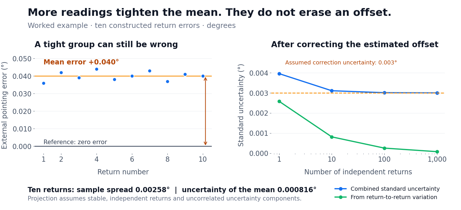
Ten constructed pointing errors cluster around positive 0.040 degrees. A second plot shows averaging approaching a correction-uncertainty floor. — The worked example separates return spread, mean offset and the uncertainty that remains after correction.

Consider a constructed calculation for ten returns to a commanded angle of 30.000°. A return means moving away, then commanding the same angle again. The values below are external pointing errors: independently measured angle minus commanded angle. They are chosen for this example; they are not product test results.

The errors, in degrees, are 0.036, 0.042, 0.039, 0.044, 0.038, 0.040, 0.043, 0.037, 0.041 and 0.040. Each return is close to the others. None is close to zero error.

The mean error is +0.040°. The sample standard deviation, which describes return-to-return spread, is 0.00258°. Assume for this calculation that conditions stay fixed, returns are independent and reference error is negligible.

Here, standard uncertainty is expressed as a standard deviation; it is not a guaranteed error limit. Under those assumptions, the standard uncertainty contributed by variation to the mean is:

u(mean) = s / √n = 0.00258° / √10 = 0.000816°.

This is the repeated-observation calculation in NIST’s uncertainty guidance, Appendix A.4. The smaller value tells us that the average error is estimated more tightly. It does not say that an individual return now has a spread of 0.000816°. Nor has averaging moved the mean toward zero: it remains +0.040°.

A correction based on the estimated offset would be −0.040°. Applied to these same data, it centres their mean by construction. That is not an independent demonstration that the correction will work on tomorrow’s returns. Validate it with fresh observations, and preserve the load, angular range and environmental conditions under which it is meant to apply.

The useful question is therefore not “How many digits can I average?” It is “Which part of the error does averaging actually address?”

Averaging improves the estimate of the mean; it does not improve every individual return.

The uncertainty that more samples cannot remove

A calibration correction is an estimate, too. Its value depends on the reference instrument, alignment and calibration procedure. Applying the correction does not remove uncertainty about it. NIST’s combined-uncertainty guidance treats that remaining uncertainty separately from the error being corrected.

Extend the calculation by assuming a standard uncertainty of 0.003° for an independently established correction. Keep the return spread at 0.00258°. If these contributions are uncorrelated, combine them as:

u(combined) = √[(0.00258° / √n)² + (0.003°)²].

Independent returns averaged	Combined standard uncertainty
10	0.00311°
100	0.00301°
1,000	0.00300°

A hundredfold increase in samples barely changes the result because uncertainty in the correction now dominates. These are projected calculations, not additional observations. Improve the reference or calibration procedure if that contribution limits the decision.

The square-root rule has another condition: the returns must provide independent information about a stable quantity. Temperature drift or slow mechanical relaxation can make adjacent results move together. A long list of readings can then exaggerate how much information was collected. Plot error against time; investigate trends and correlation before using s/√n. A correlation check is useful, but does not prove every statistical assumption. NIST’s autocorrelation guide explains this limitation.

There is one valuable exception to the slogan that averaging cannot reduce systematic effects. Measurements deliberately made in different instrument orientations can cancel certain errors. A 2025 NIST angular-calibration study describes preliminary polygon measurements and proposes averaging different instrument orientations to reduce certain systematic effects. The benefit comes from changing the measurement geometry in a controlled way—not simply repeating the same biased observation.

More samples help only the uncertainty components that the sampling procedure can reduce.

Turn a specification into a repeatable test

A field telescope sits on a metal bracket and rotary bearing, with a service cable anchored to the fixed pier in low sunlight. — The optical direction depends on the mounted structure and cable as well as the angle axis.

Imagine a camera scanning between two inspection points. It returns consistently when approaching clockwise, but its average changes after reversing direction. That pattern is worth investigating separately from random scatter. Direction-dependent effects can arise in the drive or installation; the test needs to capture them before they are hidden inside one average.

Use several angles across the working range. At each angle, record repeated returns from both directions, actual timestamps and a defined settling interval. Keep the two approach directions separate when reporting their mean errors and spreads. Repeat with the intended payload mass, centre-of-mass position, cable routing and mounting support.

The field scene shows why the measurement boundary matters. The camera’s optical direction depends on everything between its optics and the fixed support. A shaft encoder alone does not establish how the bracket, support or cable behave as conditions change. Temperature-dependent errors may be characterized and compensated within validated conditions; they are not automatically permanent or automatically removable.

For a concrete reading exercise, the Inventra S³ PED10 specification table lists 0.002° axis resolution and 0.04° accuracy as separate entries. Their twenty-to-one ratio is not a repeatability measurement, an uncertainty budget or a promise about a complete camera installation. Ask for the applicable configuration and test definition before using either value in a system calculation.

A useful report answers four final questions: what direction was measured, which reference established it, what statistic was reported and which conditions applied? Request the reference uncertainty and any correction used. Then connect the angular result to your application through the target-location error budget. A meaningful comparison starts with matching definitions and test conditions, not matching decimal places.

Compare the complete measurement, including reference, direction, load and time.

Download the full article (PDF)

Why a Repeatable Positioner Can Still Point Wrong

A fine readout can describe the wrong angle

Ten returns around a large offset

The uncertainty that more samples cannot remove

Turn a specification into a repeatable test

Sources and further reading