Why 1,500 W of Cooling Does Not Mean 1,500 W at the Plug
A rack has three different watt figures: heat inside, electrical demand and heat released outside. A checked example shows how to count each one, avoid hidden losses and verify cooling where the equipment takes in air.
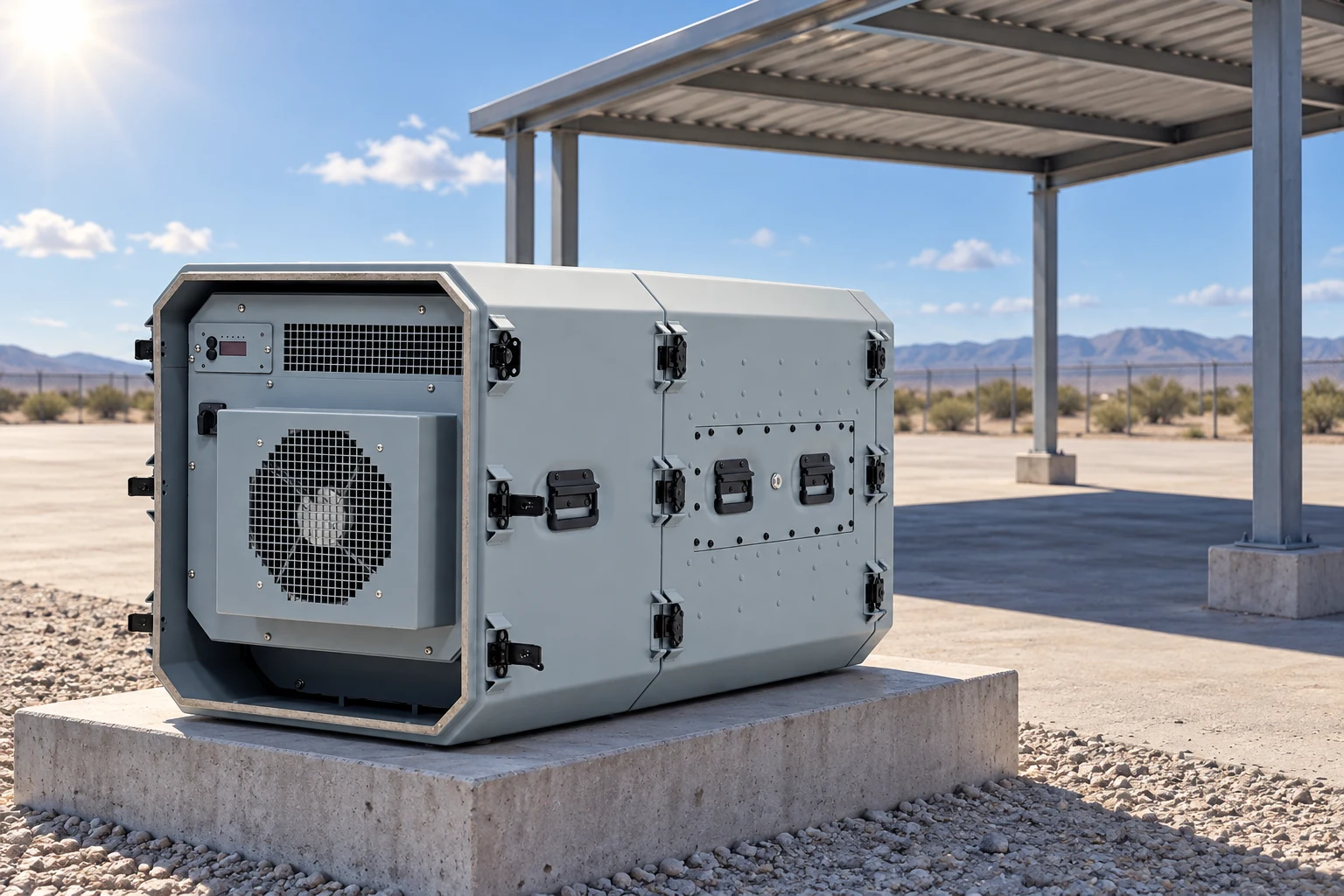
- Cooling Capacity
- 1.500 W
- Cabin Height
- 10U
- Mains Voltage
- 220 VAC
The hot side has a bigger job
In the worked example below, a cooled rack removes 960 watts of heat, draws 1,210 watts from the supply and releases 1,360 watts into its surroundings—all at the same moment. There is no contradiction. Each number measures energy crossing a different boundary. Understanding those boundaries prevents both undersized supplies and overheated installations.
The Inventra S³ ACP20 climatic rack uses vapour-compression cooling and publishes a capacity of up to 1,500 W. This describes heat removal. It does not state compressor consumption or the complete installation’s electrical demand. The linked datasheet supports the same maximum cooling figure, but does not provide the operating-point map needed for a complete power budget.
A refrigeration system moves heat from the cooled space to warmer surroundings. The compressor needs power to make that transfer possible. That input also becomes heat, so the hot side must discharge the extracted heat plus the cooling system’s own input. This follows the refrigerator energy balance.
Cooling coefficient of performance, or COP, expresses heat removed divided by power used. A cooling COP above one is possible because electricity moves heat; it is not being converted into an equal amount of “cold.” Always specify which fans and controls the quoted COP includes.
This creates a practical siting question: where will the rejected heat go? A cooling unit discharging into a small shelter can warm the very air it depends on. Sun exposure adds another load at the cabinet surface. Shade and clear heat-rejection space belong in the installation drawing, alongside the power connection.
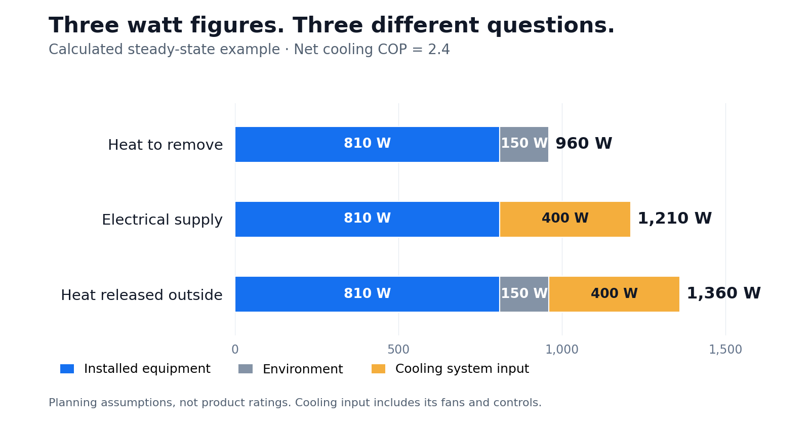
Heat removed, supply demand and rejected heat answer three different questions.
Draw the cooling boundary
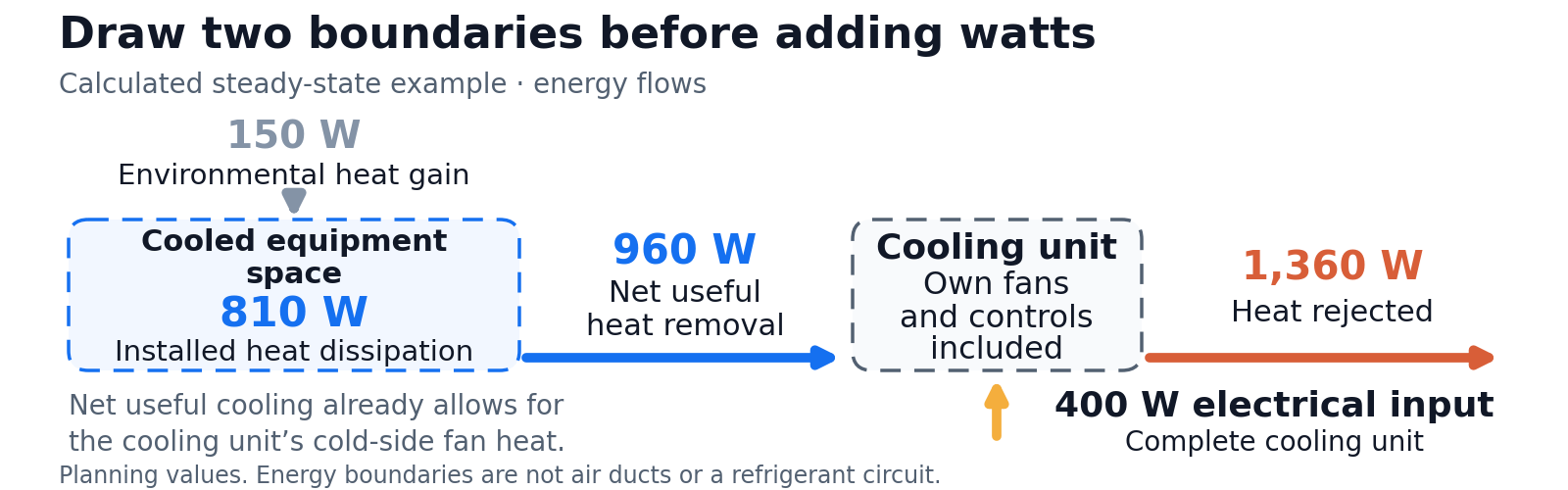
Start by drawing a line around the air space whose temperature you must control. This is the thermal boundary. For a steady operating condition, add the heat released inside that line and the heat entering through it. Do not add every electrical rating in the installation automatically.
Consider a power supply delivering 540 W to computers inside the rack at 90% efficiency. Its input is 540 ÷ 0.90 = 600 W, including 60 W of conversion loss. If the computers’ output energy remains inside, their 540 W and the supply’s 60 W both become cabinet heat. Counting 600 W at the input already covers both; adding the 60 W again would double-count it.
Move those powered loads outside the boundary and the accounting changes: only the internal supply and cable losses remain as cabinet heat. The exported power still belongs in the site electrical budget. This matters when a rack also powers a remote sensor.
| Item | Cabinet cooling budget | Site electrical budget |
|---|---|---|
| Internal electronics and conversion losses | Include heat released inside | Include their input power |
| Power delivered to an external payload | Exclude exported power | Include supplied power |
| Heat entering through cabinet walls | Include net inward heat | No direct electrical entry |
| Cooling system | Use a consistent net boundary | Include its complete input |
For an effective cabinet conductance of 6 W/K, ambient air at 45 °C and cabinet air at 30 °C give 6 × 15 = 90 W of wall gain. Conductance includes all relevant heat paths, not just the insulation panel. Thermal resistance analysis shows why metal bridges can matter. Solar gain and air leakage need separate, site-specific estimates.
A watt belongs in the cooling budget only when it becomes heat inside the chosen boundary.
One installation, three checked totals
Use the following planning values for a generic cooled rack. They are calculation inputs, not ACP20 test results. Assume steady operation, no heater demand, no significant stored-energy change and no useful power exported from the cabinet.
The internal loads are 540 W for computer circuits, 60 W of supply loss, 180 W for other equipment including its adapters, and 30 W for separate rack fans. That totals 810 W. Add the previous 90 W of wall gain and an assumed 60 W of additional net solar and air-leakage gain. Required heat removal becomes 960 W.
Now assume a net cooling COP of 2.4 at this operating point. “Net” means the cooling unit’s own cold-side fan heat has already been allowed for in its useful cooling capacity. Include all cooling-unit fans and controls in electrical input. NIST’s cooling-performance definitions show why refrigerant-side capacity and complete-unit power must not be mixed casually.
The cooler needs 960 ÷ 2.4 = 400 W. Site demand is therefore 810 + 400 = 1,210 W. The hot side releases 960 + 400 = 1,360 W. An independent check reaches the same answer: 1,210 W of electrical input plus 150 W entering from the environment equals 1,360 W leaving as heat.
A project-selected 20% cooling allowance would require 1,152 W of verified net capacity at the design condition. It would not make actual steady electrical consumption 20% higher. Keep this allowance separate from measured demand. This watt budget also does not size a breaker, cable or generator: those decisions require current, power factor, starting behaviour and the chosen equipment’s supply requirements.
960 W cooling load + 400 W cooler input = 1,360 W released outside.
Prove the capacity where the air enters
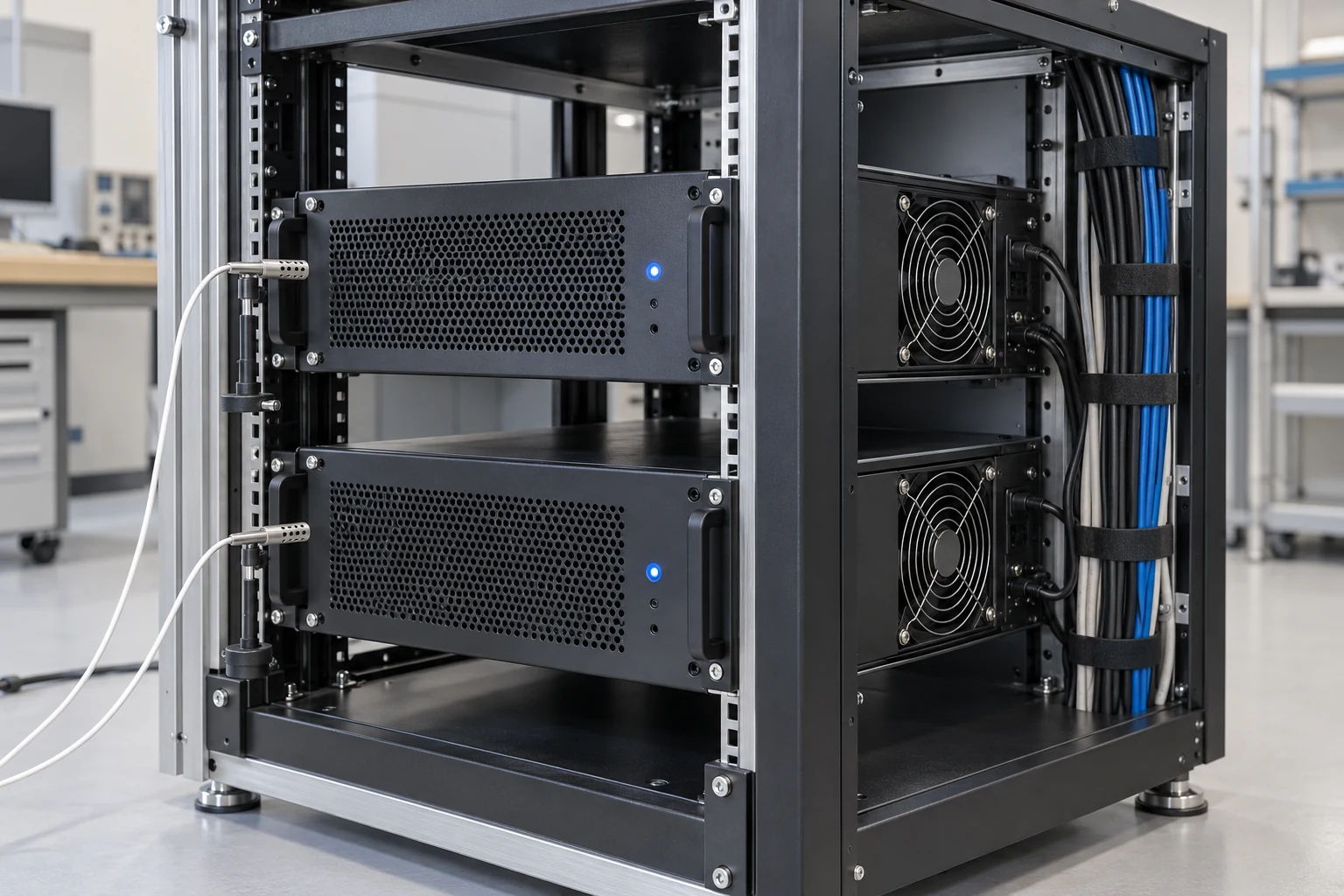
A maximum cooling figure is not a capacity curve. Ask for net available cooling and complete electrical input at the intended ambient temperature, cabinet setpoint and configuration. Confirm whether the capacity is sensible cooling—the portion that controls air temperature—or includes moisture removal. Do not assume a stated environmental qualification proves maximum cooling output at that temperature.
Lowering the setpoint is not automatically a better solution. In the wall example, moving from 30 °C to 25 °C while ambient remains 45 °C raises conductive gain from 90 W to 120 W. The refrigerator must also lift heat across a larger temperature difference. The ideal refrigeration relation explains that efficiency penalty; it cannot supply a real unit’s COP or derating curve.
Then inspect the installed equipment. A cool cabinet sensor can coexist with a warm equipment inlet if hot exhaust returns to it. Another failure is bypass: cooled air takes a gap around the equipment instead of passing through it. These are distinct mechanisms described in ASHRAE’s air-distribution guidance. More nominal cooling does not prove either one has been fixed.
Map each device’s actual intake and exhaust; some equipment uses side airflow. Keep cables and nearby panels out of those paths. Place temperature probes immediately ahead of representative inlets, including the highest-load device and any inlet near a potential exhaust return. Check the rack with its service doors and panels in their normal operating positions.
Run a representative sustained workload until temperatures settle. Record the highest inlet temperature, cabinet reading, ambient condition and complete supply demand together. Compare each inlet with that device’s limit. The useful acceptance record connects the heat budget, the cooling curve and the temperatures the electronics actually experience.
If one inlet is hot, first inspect its air path and retest after one controlled routing or separation change. If many inlets are high, compare measured workload, ambient and setpoint with the verified capacity map, then check shared heat-rejection restrictions. Treat these as diagnostic priorities. Repeat the same workload with panels in their normal positions.
A capacity calculation passes only when every relevant equipment inlet stays within its own limit.
Download the full article (PDF)
Related reading: Power Is Back. Why Is the Rack Still Getting Hotter? · The Battery Reads 24 V. Why Does the Camera Still Restart?
Sources and further reading
- ACP20 — Portable Climatic Rack Cabin
- ACP20 — Portable Climatic Rack Cabins: Datasheet
- Thermodynamics and Propulsion, Section 3.4: Refrigerators and Heat Pumps
- Thermodynamics and Propulsion, Section 16.4: Thermal Resistance Circuits
- 2019 ASHRAE Handbook, Chapter 20: Data Centres and Telecommunication Facilities
- NIST Technical Note 1848: Sensitivity Analysis of Installation Faults on Heat Pump Performance